Introduction to derfinderPlot
Leonardo Collado-Torres
Lieber Institute for Brain Development, Johns Hopkins Medical CampusCenter for Computational Biology, Johns Hopkins Universitylcolladotor@gmail.com
31 March 2026
Source:vignettes/derfinderPlot.Rmd
derfinderPlot.RmdBasics
Install derfinderPlot
R is an open-source statistical environment which can be
easily modified to enhance its functionality via packages. derfinderPlot
is a R package available via the Bioconductor
repository for packages. R can be installed on any
operating system from CRAN
after which you can install derfinderPlot
by using the following commands in your R session:
if (!requireNamespace("BiocManager", quietly = TRUE)) {
    install.packages("BiocManager")
}

BiocManager::install("derfinderPlot")

## Check that you have a valid Bioconductor installation
BiocManager::valid()
Required knowledge
derfinderPlot is based on many other packages and in particular in those that have implemented the infrastructure needed for dealing with RNA-seq data. A derfinderPlot user is not expected to deal with those packages directly but will need to be familiar with derfinder and for some plots with ggbio.
If you are asking yourself the question “Where do I start using Bioconductor?” you might be interested in this blog post.
Asking for help
As package developers, we try to explain clearly how to use our
packages and in which order to use the functions. But R and
Bioconductor have a steep learning curve so it is critical
to learn where to ask for help. The blog post quoted above mentions some
but we would like to highlight the Bioconductor support site
as the main resource for getting help: remember to use the
derfinder or derfinderPlot tags and check the older
posts. Other alternatives are available such as creating GitHub
issues and tweeting. However, please note that if you want to receive
help you should adhere to the posting
guidelines. It is particularly critical that you provide a small
reproducible example and your session information so package developers
can track down the source of the error.
Citing derfinderPlot
We hope that derfinderPlot will be useful for your research. Please use the following information to cite the package and the overall approach. Thank you!
## Citation info
citation("derfinderPlot")
## To cite package 'derfinderPlot' in publications use:
##
## Collado-Torres L, Jaffe AE, Leek JT (2017). _derfinderPlot: Plotting
## functions for derfinder_. doi:10.18129/B9.bioc.derfinderPlot
## <https://doi.org/10.18129/B9.bioc.derfinderPlot>.
## https://github.com/leekgroup/derfinderPlot - R package version
## 1.45.0, <http://www.bioconductor.org/packages/derfinderPlot>.
##
## Collado-Torres L, Nellore A, Frazee AC, Wilks C, Love MI, Langmead B,
## Irizarry RA, Leek JT, Jaffe AE (2017). "Flexible expressed region
## analysis for RNA-seq with derfinder." _Nucl. Acids Res._.
## doi:10.1093/nar/gkw852 <https://doi.org/10.1093/nar/gkw852>.
## <http://nar.oxfordjournals.org/content/early/2016/09/29/nar.gkw852>.
##
## To see these entries in BibTeX format, use 'print(<citation>,
## bibtex=TRUE)', 'toBibtex(.)', or set
## 'options(citation.bibtex.max=999)'.Introduction to derfinderPlot
derfinderPlot (Collado-Torres, Jaffe, and Leek, 2017) is an addon package for derfinder (Collado-Torres, Nellore, Frazee, Wilks, Love, Langmead, Irizarry, Leek, and Jaffe, 2017) with functions that allow you to visualize the results.
While the functions in derfinderPlot
assume you generated the data with derfinder,
they can be used with other GRanges objects properly
formatted.
The functions in derfinderPlot are:
-
plotCluster()is a tailored ggbio (Yin, Cook, and Lawrence, 2012) plot that shows all the regions in a cluster (defined by distance). It shows the base-level coverage for each sample as well as the mean for each group. If these regions overlap any known gene, the gene and the transcript annotation is displayed. -
plotOverview()is another tailored ggbio (Yin, Cook, and Lawrence, 2012) plot showing an overview of the whole genome. This plot can be useful to observe if the regions are clustered in a subset of a chromosome. It can also be used to check whether the regions match predominantly one part of the gene structure (for example, 3’ overlaps). -
plotRegionCoverage()is a fast plotting function usingRbase graphics that shows the base-level coverage for each sample inside a specific region of the genome. If the region overlaps any known gene or intron, the information is displayed. Optionally, it can display the known transcripts. This function is most likely the easiest to use withGRangesobjects from other packages.
Example
As an example, we will analyze a small subset of the samples from the BrainSpan Atlas of the Human Brain (BrainSpan, 2011) publicly available data.
We first load the required packages.
## Load libraries
suppressPackageStartupMessages(library("derfinder"))
library("derfinderData")
library("derfinderPlot")
Analyze data
For this example, we created a small table with the relevant phenotype data for 12 samples: 6 from fetal samples and 6 from adult samples. We chose at random a brain region, in this case the primary auditory cortex (core) and for the example we will only look at data from chromosome 21. Other variables include the age in years and the gender. The data is shown below.
library("knitr")
## Get pheno table
pheno <- subset(brainspanPheno, structure_acronym == "A1C")

## Display the main information
p <- pheno[, -which(colnames(pheno) %in% c(
    "structure_acronym",
    "structure_name", "file"
))]
rownames(p) <- NULL
kable(p, format = "html", row.names = TRUE)| gender | lab | Age | group | |
|---|---|---|---|---|
| 1 | M | HSB114.A1C | -0.5192308 | fetal |
| 2 | M | HSB103.A1C | -0.5192308 | fetal |
| 3 | M | HSB178.A1C | -0.4615385 | fetal |
| 4 | M | HSB154.A1C | -0.4615385 | fetal |
| 5 | F | HSB150.A1C | -0.5384615 | fetal |
| 6 | F | HSB149.A1C | -0.5192308 | fetal |
| 7 | F | HSB130.A1C | 21.0000000 | adult |
| 8 | M | HSB136.A1C | 23.0000000 | adult |
| 9 | F | HSB126.A1C | 30.0000000 | adult |
| 10 | M | HSB145.A1C | 36.0000000 | adult |
| 11 | M | HSB123.A1C | 37.0000000 | adult |
| 12 | F | HSB135.A1C | 40.0000000 | adult |
We can load the data from derfinderData
(Collado-Torres, Jaffe, and Leek, 2025) by first identifying the paths
to the BigWig files with derfinder::rawFiles() and then
loading the data with derfinder::fullCoverage().
## Determine the files to use and fix the names
files <- rawFiles(system.file("extdata", "A1C", package = "derfinderData"),
    samplepatt = "bw", fileterm = NULL
)
names(files) <- gsub(".bw", "", names(files))

## Load the data from disk
system.time(fullCov <- fullCoverage(files = files, chrs = "chr21"))
## 2026-03-31 17:51:55.03888 fullCoverage: processing chromosome chr21## 2026-03-31 17:51:55.051432 loadCoverage: finding chromosome lengths## 2026-03-31 17:51:55.073089 loadCoverage: loading BigWig file /__w/_temp/Library/derfinderData/extdata/A1C/HSB103.bw## 2026-03-31 17:51:55.228545 loadCoverage: loading BigWig file /__w/_temp/Library/derfinderData/extdata/A1C/HSB114.bw## 2026-03-31 17:51:55.365388 loadCoverage: loading BigWig file /__w/_temp/Library/derfinderData/extdata/A1C/HSB123.bw## 2026-03-31 17:51:55.466864 loadCoverage: loading BigWig file /__w/_temp/Library/derfinderData/extdata/A1C/HSB126.bw## 2026-03-31 17:51:55.53811 loadCoverage: loading BigWig file /__w/_temp/Library/derfinderData/extdata/A1C/HSB130.bw## 2026-03-31 17:51:55.630594 loadCoverage: loading BigWig file /__w/_temp/Library/derfinderData/extdata/A1C/HSB135.bw## 2026-03-31 17:51:55.698533 loadCoverage: loading BigWig file /__w/_temp/Library/derfinderData/extdata/A1C/HSB136.bw## 2026-03-31 17:51:55.770109 loadCoverage: loading BigWig file /__w/_temp/Library/derfinderData/extdata/A1C/HSB145.bw## 2026-03-31 17:51:55.85898 loadCoverage: loading BigWig file /__w/_temp/Library/derfinderData/extdata/A1C/HSB149.bw## 2026-03-31 17:51:55.94791 loadCoverage: loading BigWig file /__w/_temp/Library/derfinderData/extdata/A1C/HSB150.bw## 2026-03-31 17:51:56.019534 loadCoverage: loading BigWig file /__w/_temp/Library/derfinderData/extdata/A1C/HSB154.bw## 2026-03-31 17:51:56.125102 loadCoverage: loading BigWig file /__w/_temp/Library/derfinderData/extdata/A1C/HSB178.bw## 2026-03-31 17:51:56.227252 loadCoverage: applying the cutoff to the merged data## 2026-03-31 17:51:56.249099 filterData: originally there were 48129895 rows, now there are 48129895 rows. Meaning that 0 percent was filtered.## user system elapsed
## 1.218 0.038 1.256Alternatively, since the BigWig files are publicly available from
BrainSpan (see here),
we can extract the relevant coverage data using
derfinder::fullCoverage(). Note that as of rtracklayer
1.25.16 BigWig files are not supported on Windows: you can find the
fullCov object inside derfinderData
to follow the examples.
## Determine the files to use and fix the names
files <- pheno$file
names(files) <- gsub(".A1C", "", pheno$lab)

## Load the data from the web
system.time(fullCov <- fullCoverage(files = files, chrs = "chr21"))
Once we have the base-level coverage data for all 12 samples, we can construct the models. In this case, we want to find differences between fetal and adult samples while adjusting for gender and a proxy of the library size.
## Get some idea of the library sizes
sampleDepths <- sampleDepth(collapseFullCoverage(fullCov), 1)
## 2026-03-31 17:51:56.457992 sampleDepth: Calculating sample quantiles## 2026-03-31 17:51:56.538645 sampleDepth: Calculating sample adjustments
## Define models
models <- makeModels(sampleDepths,
    testvars = pheno$group,
    adjustvars = pheno[, c("gender")]
)
Next, we can find candidate differentially expressed regions (DERs) using as input the segments of the genome where at least one sample has coverage greater than 3. In this particular example, we chose a low theoretical F-statistic cutoff and used 20 permutations.
## Filter coverage
filteredCov <- lapply(fullCov, filterData, cutoff = 3)
## 2026-03-31 17:51:57.62273 filterData: originally there were 48129895 rows, now there are 90023 rows. Meaning that 99.81 percent was filtered.
## Perform differential expression analysis
suppressPackageStartupMessages(library("bumphunter"))
system.time(results <- analyzeChr(
    chr = "chr21", filteredCov$chr21,
    models, groupInfo = pheno$group, writeOutput = FALSE,
    cutoffFstat = 5e-02, nPermute = 20, seeds = 20140923 + seq_len(20)
))
## 2026-03-31 17:51:58.51422 analyzeChr: Pre-processing the coverage data## 2026-03-31 17:51:59.851174 analyzeChr: Calculating statistics## 2026-03-31 17:51:59.853724 calculateStats: calculating the F-statistics## 2026-03-31 17:51:59.968506 analyzeChr: Calculating pvalues## 2026-03-31 17:51:59.96903 analyzeChr: Using the following theoretical cutoff for the F-statistics 5.31765507157871## 2026-03-31 17:51:59.969947 calculatePvalues: identifying data segments## 2026-03-31 17:51:59.975419 findRegions: segmenting information## 2026-03-31 17:51:59.997277 findRegions: identifying candidate regions## 2026-03-31 17:52:00.03402 findRegions: identifying region clusters## 2026-03-31 17:52:00.141166 calculatePvalues: calculating F-statistics for permutation 1 and seed 20140924## 2026-03-31 17:52:00.241784 findRegions: segmenting information## 2026-03-31 17:52:00.260034 findRegions: identifying candidate regions## 2026-03-31 17:52:00.301637 calculatePvalues: calculating F-statistics for permutation 2 and seed 20140925## 2026-03-31 17:52:00.403671 findRegions: segmenting information## 2026-03-31 17:52:00.422265 findRegions: identifying candidate regions## 2026-03-31 17:52:00.452937 calculatePvalues: calculating F-statistics for permutation 3 and seed 20140926## 2026-03-31 17:52:00.554338 findRegions: segmenting information## 2026-03-31 17:52:00.572982 findRegions: identifying candidate regions## 2026-03-31 17:52:00.603668 calculatePvalues: calculating F-statistics for permutation 4 and seed 20140927## 2026-03-31 17:52:00.705135 findRegions: segmenting information## 2026-03-31 17:52:00.723913 findRegions: identifying candidate regions## 2026-03-31 17:52:00.755189 calculatePvalues: calculating F-statistics for permutation 5 and seed 20140928## 2026-03-31 17:52:00.855366 findRegions: segmenting information## 2026-03-31 17:52:00.873356 findRegions: identifying candidate regions## 2026-03-31 17:52:00.903844 calculatePvalues: calculating F-statistics for permutation 6 and seed 20140929## 2026-03-31 17:52:01.005022 findRegions: segmenting information## 2026-03-31 17:52:01.023655 findRegions: identifying candidate regions## 2026-03-31 17:52:01.054294 calculatePvalues: calculating F-statistics for permutation 7 and seed 20140930## 2026-03-31 17:52:01.157952 findRegions: segmenting information## 2026-03-31 17:52:01.176545 findRegions: identifying candidate regions## 2026-03-31 17:52:01.206921 calculatePvalues: calculating F-statistics for permutation 8 and seed 20140931## 2026-03-31 17:52:01.308403 findRegions: segmenting information## 2026-03-31 17:52:01.327206 findRegions: identifying candidate regions## 2026-03-31 17:52:01.357925 calculatePvalues: calculating F-statistics for permutation 9 and seed 20140932## 2026-03-31 17:52:01.458419 findRegions: segmenting information## 2026-03-31 17:52:01.477011 findRegions: identifying candidate regions## 2026-03-31 17:52:01.507913 calculatePvalues: calculating F-statistics for permutation 10 and seed 20140933## 2026-03-31 17:52:02.401301 findRegions: segmenting information## 2026-03-31 17:52:02.420042 findRegions: identifying candidate regions## 2026-03-31 17:52:02.450516 calculatePvalues: calculating F-statistics for permutation 11 and seed 20140934## 2026-03-31 17:52:02.548522 findRegions: segmenting information## 2026-03-31 17:52:02.567153 findRegions: identifying candidate regions## 2026-03-31 17:52:02.598169 calculatePvalues: calculating F-statistics for permutation 12 and seed 20140935## 2026-03-31 17:52:02.69875 findRegions: segmenting information## 2026-03-31 17:52:02.717362 findRegions: identifying candidate regions## 2026-03-31 17:52:02.747734 calculatePvalues: calculating F-statistics for permutation 13 and seed 20140936## 2026-03-31 17:52:02.840873 findRegions: segmenting information## 2026-03-31 17:52:02.859477 findRegions: identifying candidate regions## 2026-03-31 17:52:02.895236 calculatePvalues: calculating F-statistics for permutation 14 and seed 20140937## 2026-03-31 17:52:02.986962 findRegions: segmenting information## 2026-03-31 17:52:03.005446 findRegions: identifying candidate regions## 2026-03-31 17:52:03.035669 calculatePvalues: calculating F-statistics for permutation 15 and seed 20140938## 2026-03-31 17:52:03.134877 findRegions: segmenting information## 2026-03-31 17:52:03.15344 findRegions: identifying candidate regions## 2026-03-31 17:52:03.183712 calculatePvalues: calculating F-statistics for permutation 16 and seed 20140939## 2026-03-31 17:52:03.284523 findRegions: segmenting information## 2026-03-31 17:52:03.303228 findRegions: identifying candidate regions## 2026-03-31 17:52:03.334332 calculatePvalues: calculating F-statistics for permutation 17 and seed 20140940## 2026-03-31 17:52:03.434294 findRegions: segmenting information## 2026-03-31 17:52:03.452944 findRegions: identifying candidate regions## 2026-03-31 17:52:03.48331 calculatePvalues: calculating F-statistics for permutation 18 and seed 20140941## 2026-03-31 17:52:03.575667 findRegions: segmenting information## 2026-03-31 17:52:03.594253 findRegions: identifying candidate regions## 2026-03-31 17:52:03.624701 calculatePvalues: calculating F-statistics for permutation 19 and seed 20140942## 2026-03-31 17:52:03.723029 findRegions: segmenting information## 2026-03-31 17:52:03.741672 findRegions: identifying candidate regions## 2026-03-31 17:52:03.772249 calculatePvalues: calculating F-statistics for permutation 20 and seed 20140943## 2026-03-31 17:52:03.864692 findRegions: segmenting information## 2026-03-31 17:52:03.88269 findRegions: identifying candidate regions## 2026-03-31 17:52:03.928858 calculatePvalues: calculating the p-values## 2026-03-31 17:52:03.974126 analyzeChr: Annotating regions## No annotationPackage supplied. Trying org.Hs.eg.db.## Loading required package: org.Hs.eg.db## Loading required package: AnnotationDbi## Loading required package: Biobase## Welcome to Bioconductor
##
## Vignettes contain introductory material; view with
## 'browseVignettes()'. To cite Bioconductor, see
## 'citation("Biobase")', and for packages 'citation("pkgname")'.## ## Getting TSS and TSE.## Getting CSS and CSE.## Warning in .set_group_names(grl, use.names, txdb, by): some group names are NAs
## or duplicated## Getting exons.## Warning in .set_group_names(grl, use.names, txdb, by): some group names are NAs
## or duplicated## Annotating genes.## ...## user system elapsed
## 50.895 2.633 50.949
## Quick access to the results
regions <- results$regions$regions

## Annotation database to use
suppressPackageStartupMessages(library("TxDb.Hsapiens.UCSC.hg19.knownGene"))
txdb <- TxDb.Hsapiens.UCSC.hg19.knownGene
plotOverview()
Now that we have obtained the main results using derfinder,
we can proceed to visualizing the results using derfinderPlot.
The easiest to use of all the functions is plotOverview()
which takes a set of regions and annotation information produced by
bumphunter::matchGenes().
Figure @ref(fig:plotOverview) shows the candidate DERs colored by whether their q-value was less than 0.10 or not.
## Q-values overview
plotOverview(regions = regions, annotation = results$annotation, type = "qval")
## 2026-03-31 17:52:49.610896 plotOverview: assigning chromosome lengths from hg19!## Scale for x is already present.
## Adding another scale for x, which will replace the existing scale.
## Scale for x is already present.
## Adding another scale for x, which will replace the existing scale.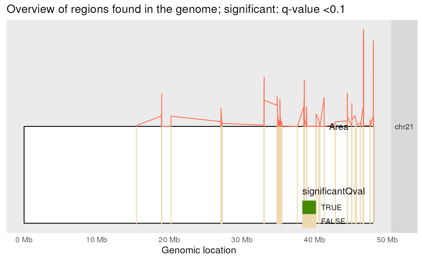
Location of the DERs in the genome. This plot is was designed for many chromosomes but only one is shown here for simplicity.
Figure @ref(fig:plotOverview2) shows the candidate DERs colored by the type of gene feature they are nearest too.
## Annotation overview
plotOverview(
    regions = regions, annotation = results$annotation,
    type = "annotation"
)
## 2026-03-31 17:52:50.597719 plotOverview: assigning chromosome lengths from hg19!## Scale for x is already present.
## Adding another scale for x, which will replace the existing scale.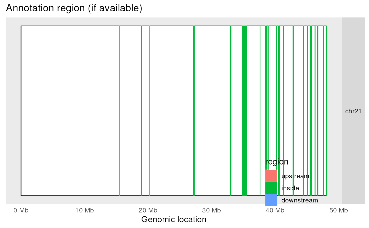
Location of the DERs in the genome and colored by annotation class. This plot is was designed for many chromosomes but only one is shown here for simplicity.
In this particular example, because we are only using data from one chromosome the above plot is not as informative as in a real case scenario. However, with this plot we can quickly observe that nearly all of the candidate DERs are inside an exon.
plotRegionCoverage()
The complete opposite of visualizing the candidate DERs at the
genome-level is to visualize them one region at a time.
plotRegionCoverage() allows us to do this quickly for a
large number of regions.
Before using this function, we need to process more detailed
information using two derfinder
functions: annotateRegions() and
getRegionCoverage() as shown below.
## Get required information for the plots
annoRegs <- annotateRegions(regions, genomicState$fullGenome)
## 2026-03-31 17:52:51.372025 annotateRegions: counting## 2026-03-31 17:52:51.427093 annotateRegions: annotating
regionCov <- getRegionCoverage(fullCov, regions)## 2026-03-31 17:52:51.510275 getRegionCoverage: processing chr21## 2026-03-31 17:52:51.552495 getRegionCoverage: done processing chr21Once we have the relevant information we can proceed to plotting the
first 10 regions. In this case, we will supply
plotRegionCoverage() with the information it needs to plot
transcripts overlapping these 10 regions (Figures @ref(fig:plotRegCov1),
@ref(fig:plotRegCov2), @ref(fig:plotRegCov3), @ref(fig:plotRegCov4),
@ref(fig:plotRegCov5), @ref(fig:plotRegCov6), @ref(fig:plotRegCov7),
@ref(fig:plotRegCov8), @ref(fig:plotRegCov9),
@ref(fig:plotRegCov10)).
## Plot top 10 regions
plotRegionCoverage(
    regions = regions, regionCoverage = regionCov,
    groupInfo = pheno$group, nearestAnnotation = results$annotation,
    annotatedRegions = annoRegs, whichRegions = 1:10, txdb = txdb, scalefac = 1,
    ask = FALSE, verbose = FALSE
)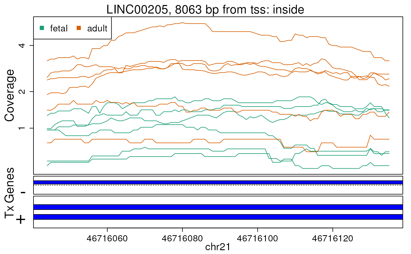
Base-pair resolution plot of differentially expressed region 1.
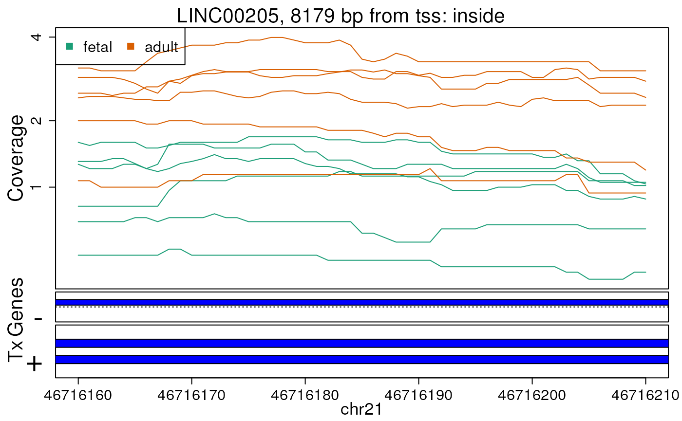
Base-pair resolution plot of differentially expressed region 2.
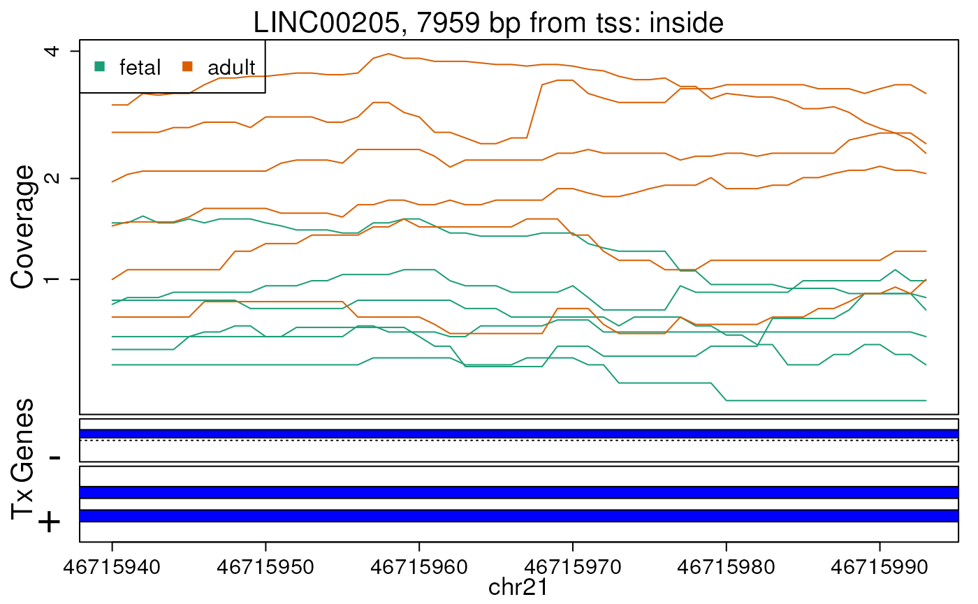
Base-pair resolution plot of differentially expressed region 3.
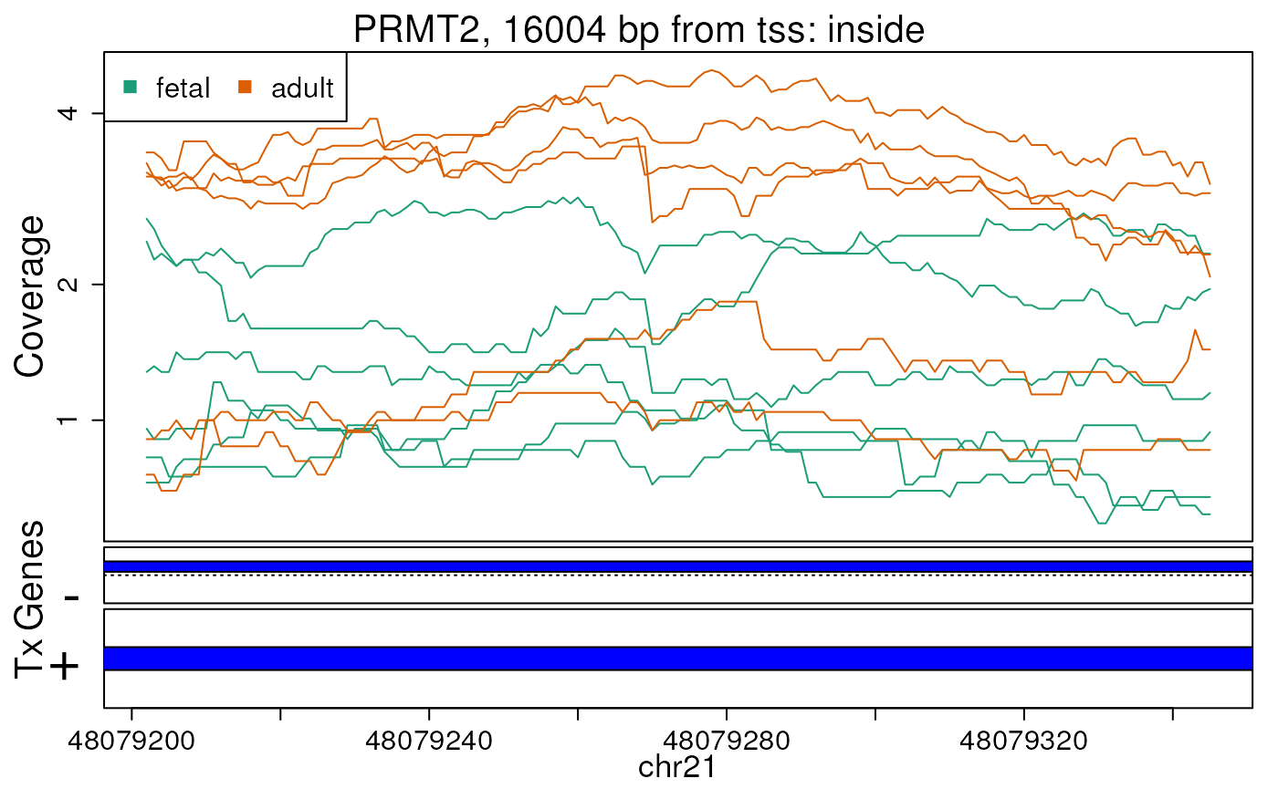
Base-pair resolution plot of differentially expressed region 4.
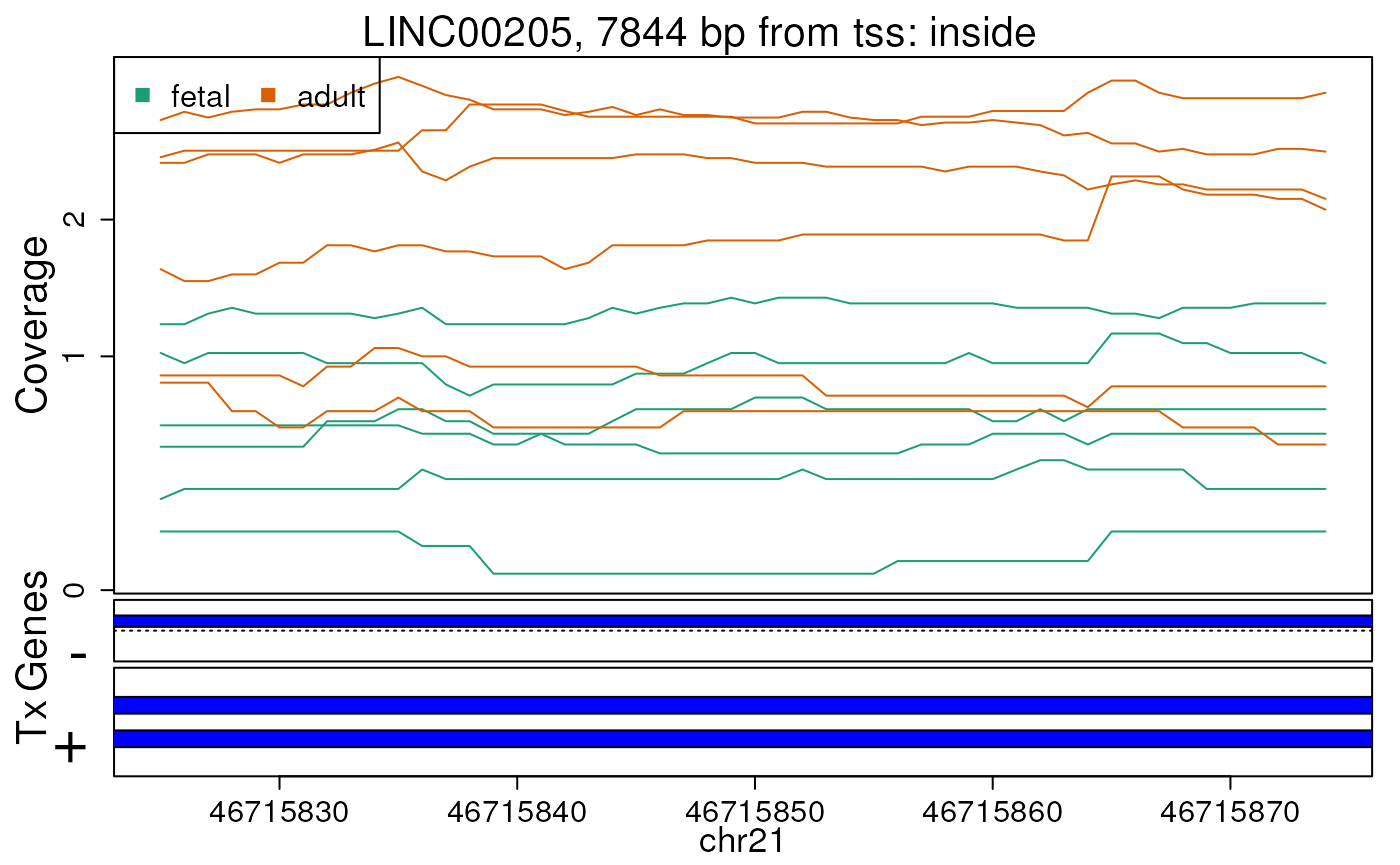
Base-pair resolution plot of differentially expressed region 5.
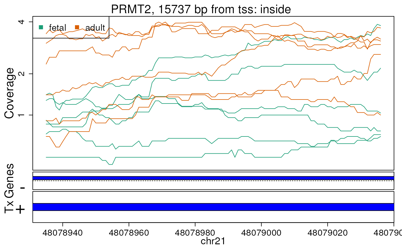
Base-pair resolution plot of differentially expressed region 6.
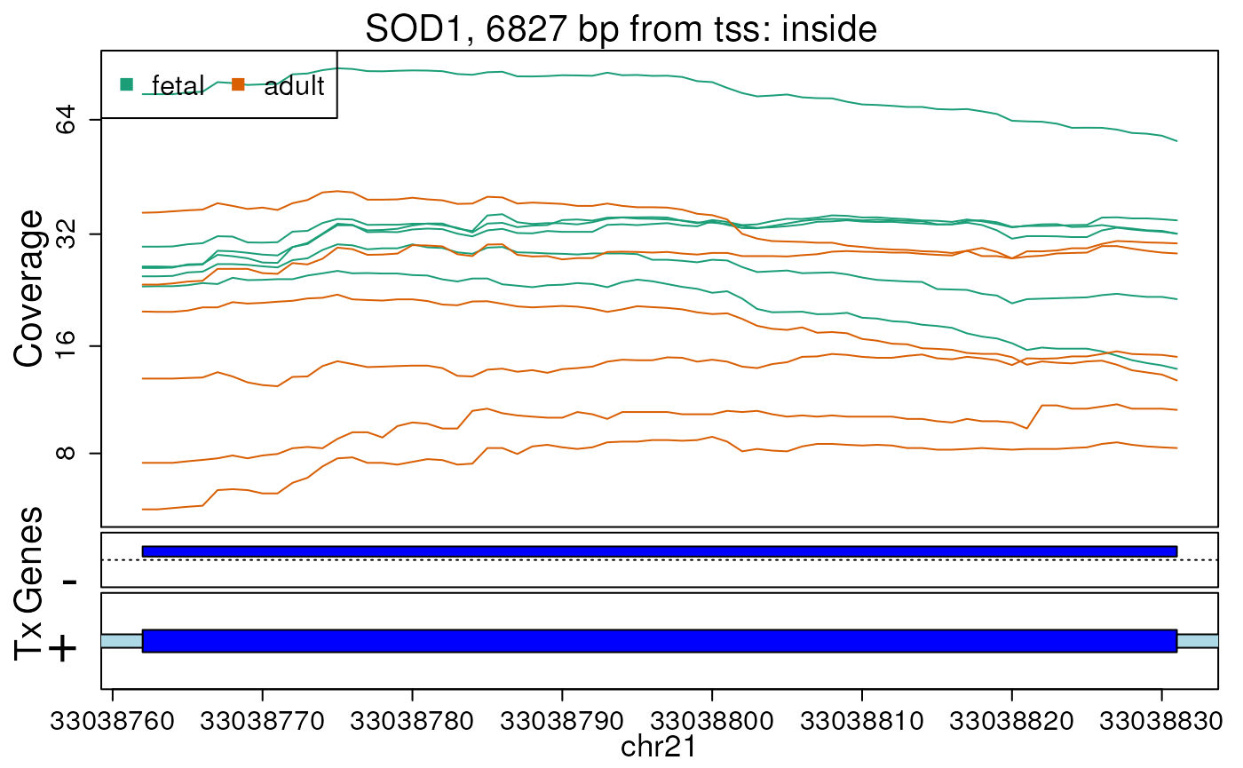
Base-pair resolution plot of differentially expressed region 7.
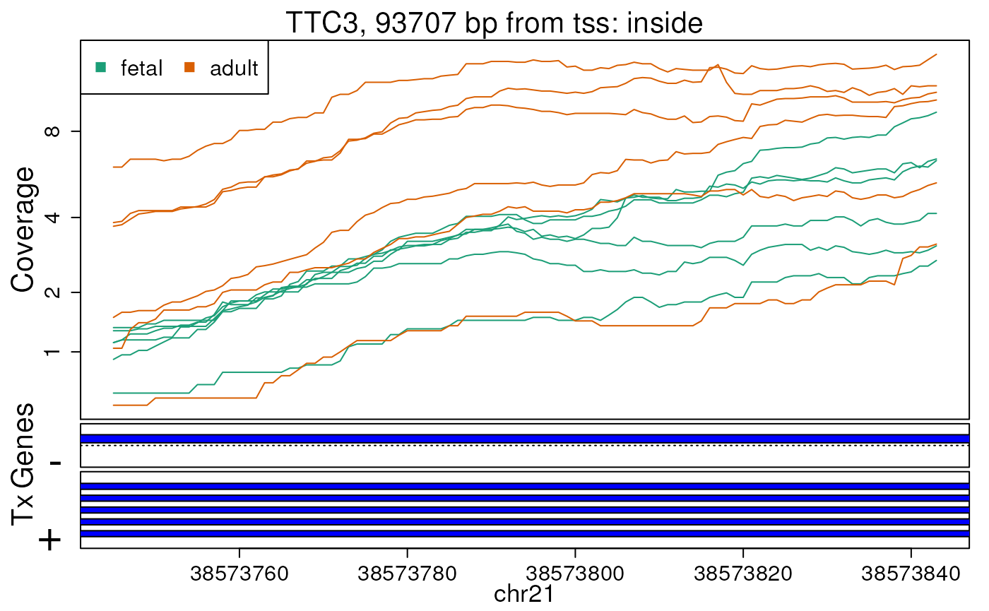
Base-pair resolution plot of differentially expressed region 8.
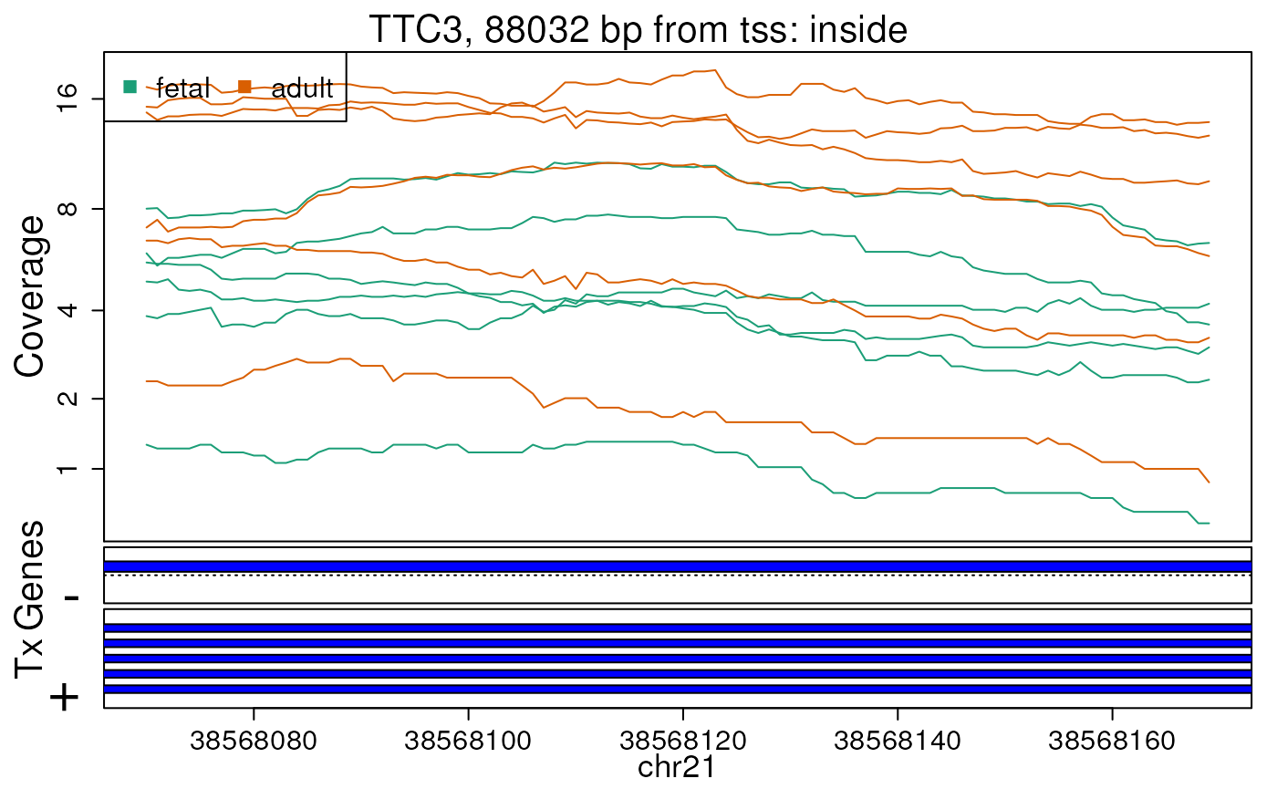
Base-pair resolution plot of differentially expressed region 9.
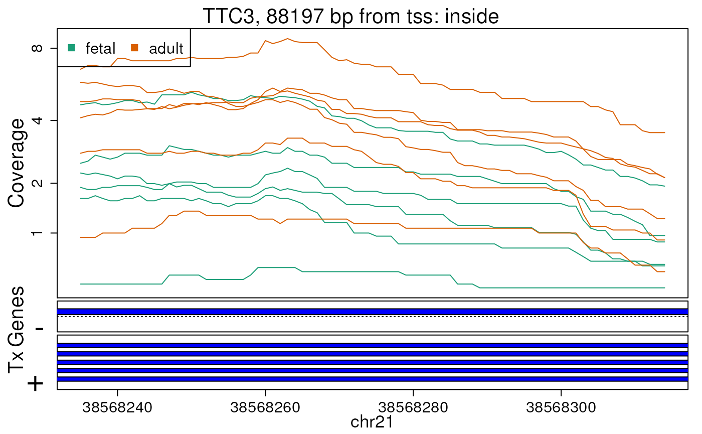
Base-pair resolution plot of differentially expressed region 10.
The base-level coverage is shown in a log2 scale with any overlapping exons shown in dark blue and known introns in light blue.
plotCluster()
In this example, we noticed with the
plotRegionCoverage() plots that most of the candidate DERs
are contained in known exons. Sometimes, the signal might be low or we
might have used very stringent cutoffs in the derfinder
analysis. One way we can observe this is by plotting clusters of regions
where a cluster is defined as regions within 300 bp (default option) of
each other.
To visualize the clusters, we can use plotCluster()
which takes similar input to plotOverview() with the
notable addition of the coverage information as well as the
idx argument. This argument specifies which region to focus
on: it will be plotted with a red bar and will determine the cluster to
display.
In Figure @ref(fig:plotCluster) we observe one large candidate DER with other nearby ones that do not have a q-value less than 0.10. In a real analysis, we would probably discard this region as the coverage is fairly low.
## First cluster
plotCluster(
    idx = 1, regions = regions, annotation = results$annotation,
    coverageInfo = fullCov$chr21, txdb = txdb, groupInfo = pheno$group,
    titleUse = "pval"
)
## Parsing transcripts...## Parsing exons...## Parsing cds...## Parsing utrs...## ------exons...## ------cdss...## ------introns...## ------utr...## aggregating...## Done## Constructing graphics...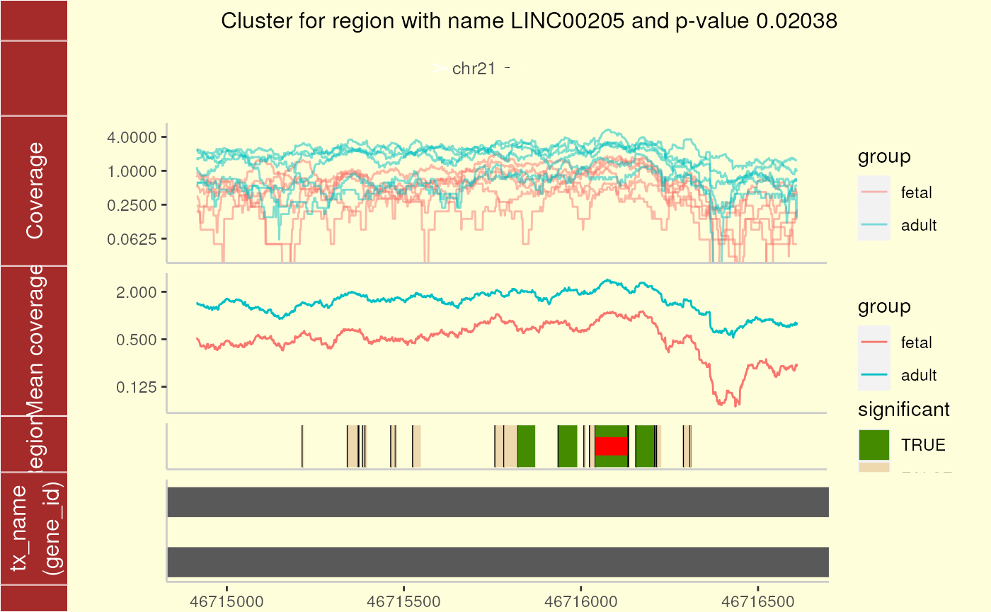
Cluster plot for cluster 1 using ggbio.
The second cluster (Figure @ref(fig:plotCluster2)) shows a larger number of potential DERs (again without q-values less than 0.10) in a segment of the genome where the coverage data is highly variable. This is a common occurrence with RNA-seq data.
## Second cluster
plotCluster(
    idx = 2, regions = regions, annotation = results$annotation,
    coverageInfo = fullCov$chr21, txdb = txdb, groupInfo = pheno$group,
    titleUse = "pval"
)
## Parsing transcripts...## Parsing exons...## Parsing cds...## Parsing utrs...## ------exons...## ------cdss...## ------introns...## ------utr...## aggregating...## Done## Constructing graphics...## Warning in !vapply(ggl, fixed, logical(1L)) & !vapply(PlotList, is, "Ideogram",
## : longer object length is not a multiple of shorter object length## Warning in scale_y_continuous(trans = log2_trans()): log-2
## transformation introduced infinite values.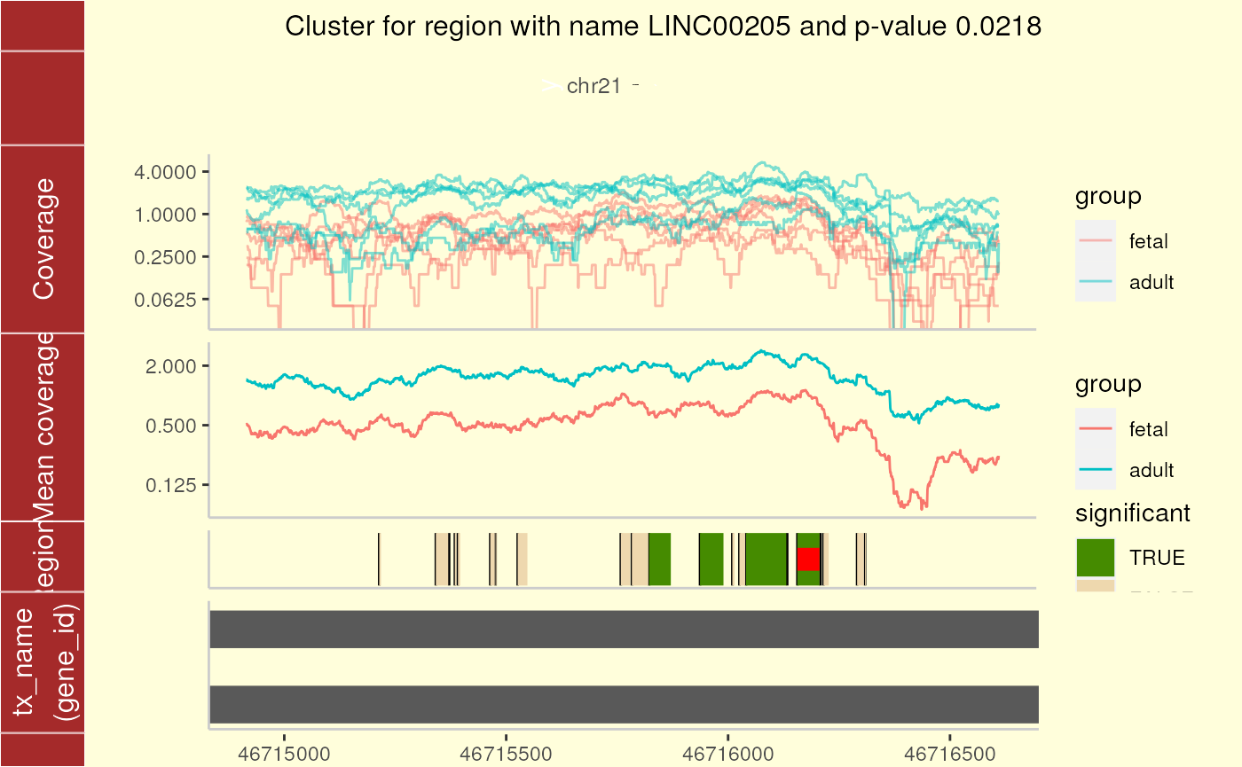
Cluster plot for cluster 2 using ggbio.
These plots show an ideogram which helps quickly identify which region of the genome we are focusing on. Then, the base-level coverage information for each sample is displayed in log2. Next, the coverage group means are shown in the log2 scale. The plot is completed with the potential and candidate DERs as well as any known transcripts.
vennRegions
derfinder
has functions for annotating regions given their genomic state. A
typical visualization is to then view how many regions overlap known
exons, introns, intergenic regions, none of them or several of these
groups in a venn diagram. The function vennRegions() makes
this plot using the output from
derfinder::annotateRegions() as shown in Figure
@ref(fig:vennRegions).
## Make venn diagram
venn <- vennRegions(annoRegs)
Venn diagram of regions by annotation class.
## It returns the actual venn counts information
venn
## exon intergenic intron Counts
## 1 0 0 0 0
## 2 0 0 1 2
## 3 0 1 0 4
## 4 0 1 1 0
## 5 1 0 0 259
## 6 1 0 1 35
## 7 1 1 0 0
## 8 1 1 1 0
## attr(,"class")
## [1] "VennCounts"Reproducibility
This package was made possible thanks to:
- R (R Core Team, 2026)
- GenomeInfoDb (Arora, Morgan, Carlson, and Pagès, 2017)
- GenomicRanges (Lawrence, Huber, Pagès, Aboyoun, Carlson, Gentleman, Morgan, and Carey, 2013)
- ggbio (Yin, Cook, and Lawrence, 2012)
- ggplot2 (Wickham, 2016)
- IRanges (Lawrence, Huber, Pagès et al., 2013)
- plyr (Wickham, 2011)
- RColorBrewer (Neuwirth, 2022)
- reshape2 (Wickham, 2007)
- scales (Wickham, Pedersen, and Seidel, 2025)
- biovizBase (Yin, Lawrence, and Cook, 2025)
- bumphunter (Jaffe, Murakami, Lee, Leek, Fallin, Feinberg, and Irizarry, 2012) and (Jaffe, Murakami, Lee, Leek, Fallin, Feinberg, and Irizarry, 2012)
- derfinder (Collado-Torres, Nellore, Frazee et al., 2017)
- derfinderData (Collado-Torres, Jaffe, and Leek, 2025)
- sessioninfo (Wickham, Chang, Flight, Müller, and Hester, 2025)
- knitr (Xie, 2014)
- BiocStyle (Oleś, 2025)
- RefManageR (McLean, 2017)
- rmarkdown (Allaire, Xie, Dervieux, McPherson, Luraschi, Ushey, Atkins, Wickham, Cheng, Chang, and Iannone, 2026)
- testthat (Wickham, 2011)
- TxDb.Hsapiens.UCSC.hg19.knownGene (Team and Maintainer, 2025)
Code for creating the vignette
## Create the vignette
library("rmarkdown")
system.time(render("derfinderPlot.Rmd", "BiocStyle::html_document"))

## Extract the R code
library("knitr")
knit("derfinderPlot.Rmd", tangle = TRUE)
## Clean up
unlink("chr21", recursive = TRUE)
Date the vignette was generated.
## [1] "2026-03-31 17:53:18 UTC"Wallclock time spent generating the vignette.
## Time difference of 1.602 minsR session information.
## ─ Session info ───────────────────────────────────────────────────────────────────────────────────────────────────────
##  setting  value
##  version  R Under development (unstable) (2026-03-28 r89738)
##  os       Ubuntu 24.04.4 LTS
##  system   x86_64, linux-gnu
##  ui       X11
##  language en
##  collate  en_US.UTF-8
##  ctype    en_US.UTF-8
##  tz       UTC
##  date     2026-03-31
##  pandoc   3.9.0.2 @ /usr/bin/ (via rmarkdown)
##  quarto   1.8.25 @ /usr/local/bin/quarto
##
## ─ Packages ───────────────────────────────────────────────────────────────────────────────────────────────────────────
##  package                           * version    date (UTC) lib source
##  abind                               1.4-8      2024-09-12 [1] CRAN (R 4.6.0)
##  AnnotationDbi                     * 1.73.0     2025-10-31 [1] Bioconductor 3.23 (R 4.6.0)
##  AnnotationFilter                    1.35.0     2025-10-31 [1] Bioconductor 3.23 (R 4.6.0)
##  backports                           1.5.0      2024-05-23 [1] CRAN (R 4.6.0)
##  base64enc                           0.1-6      2026-02-02 [2] CRAN (R 4.7.0)
##  bibtex                              0.5.2      2026-02-03 [1] CRAN (R 4.6.0)
##  Biobase                           * 2.71.0     2025-10-30 [1] Bioconductor 3.23 (R 4.6.0)
##  BiocGenerics                      * 0.57.0     2025-10-30 [1] Bioconductor 3.23 (R 4.6.0)
##  BiocIO                              1.21.0     2025-10-30 [1] Bioconductor 3.23 (R 4.6.0)
##  BiocManager                         1.30.27    2025-11-14 [2] CRAN (R 4.7.0)
##  BiocParallel                        1.45.0     2025-10-30 [1] Bioconductor 3.23 (R 4.6.0)
##  BiocStyle                         * 2.39.0     2025-10-30 [1] Bioconductor 3.23 (R 4.6.0)
##  Biostrings                          2.79.5     2026-03-06 [1] Bioconductor 3.23 (R 4.7.0)
##  biovizBase                          1.59.0     2025-11-04 [1] Bioconductor 3.23 (R 4.6.0)
##  bit                                 4.6.0      2025-03-06 [1] CRAN (R 4.6.0)
##  bit64                               4.6.0-1    2025-01-16 [1] CRAN (R 4.6.0)
##  bitops                              1.0-9      2024-10-03 [1] CRAN (R 4.6.0)
##  blob                                1.3.0      2026-01-14 [1] CRAN (R 4.6.0)
##  bookdown                            0.46       2025-12-05 [1] CRAN (R 4.6.0)
##  BSgenome                            1.79.1     2025-11-04 [1] Bioconductor 3.23 (R 4.6.0)
##  bslib                               0.10.0     2026-01-26 [2] CRAN (R 4.7.0)
##  bumphunter                        * 1.53.0     2025-11-04 [1] Bioconductor 3.23 (R 4.6.0)
##  cachem                              1.1.0      2024-05-16 [2] CRAN (R 4.7.0)
##  checkmate                           2.3.4      2026-02-03 [1] CRAN (R 4.6.0)
##  cigarillo                           1.1.0      2025-10-31 [1] Bioconductor 3.23 (R 4.6.0)
##  cli                                 3.6.5      2025-04-23 [2] CRAN (R 4.7.0)
##  cluster                             2.1.8.2    2026-02-05 [3] CRAN (R 4.7.0)
##  codetools                           0.2-20     2024-03-31 [3] CRAN (R 4.7.0)
##  colorspace                          2.1-2      2025-09-22 [1] CRAN (R 4.6.0)
##  crayon                              1.5.3      2024-06-20 [2] CRAN (R 4.7.0)
##  curl                                7.0.0      2025-08-19 [2] CRAN (R 4.7.0)
##  data.table                          1.18.2.1   2026-01-27 [1] CRAN (R 4.6.0)
##  DBI                                 1.3.0      2026-02-25 [1] CRAN (R 4.7.0)
##  DelayedArray                        0.37.0     2025-10-31 [1] Bioconductor 3.23 (R 4.6.0)
##  derfinder                         * 1.45.0     2025-11-04 [1] Bioconductor 3.23 (R 4.6.0)
##  derfinderData                     * 2.29.0     2025-10-30 [1] Bioconductor 3.23 (R 4.6.0)
##  derfinderHelper                     1.45.0     2025-10-31 [1] Bioconductor 3.23 (R 4.6.0)
##  derfinderPlot                     * 1.45.0     2026-03-31 [1] Bioconductor
##  desc                                1.4.3      2023-12-10 [2] CRAN (R 4.7.0)
##  dichromat                           2.0-0.1    2022-05-02 [1] CRAN (R 4.6.0)
##  digest                              0.6.39     2025-11-19 [2] CRAN (R 4.7.0)
##  doRNG                               1.8.6.3    2026-02-05 [1] CRAN (R 4.6.0)
##  dplyr                               1.2.0      2026-02-03 [1] CRAN (R 4.6.0)
##  ensembldb                           2.35.0     2025-11-04 [1] Bioconductor 3.23 (R 4.6.0)
##  evaluate                            1.0.5      2025-08-27 [2] CRAN (R 4.7.0)
##  farver                              2.1.2      2024-05-13 [1] CRAN (R 4.6.0)
##  fastmap                             1.2.0      2024-05-15 [2] CRAN (R 4.7.0)
##  foreach                           * 1.5.2      2022-02-02 [1] CRAN (R 4.6.0)
##  foreign                             0.8-91     2026-01-29 [3] CRAN (R 4.7.0)
##  Formula                             1.2-5      2023-02-24 [1] CRAN (R 4.6.0)
##  fs                                  2.0.1      2026-03-24 [2] CRAN (R 4.7.0)
##  generics                          * 0.1.4      2025-05-09 [1] CRAN (R 4.6.0)
##  GenomeInfoDb                        1.47.2     2025-12-04 [1] Bioconductor 3.23 (R 4.6.0)
##  GenomicAlignments                   1.47.0     2025-10-31 [1] Bioconductor 3.23 (R 4.6.0)
##  GenomicFeatures                   * 1.63.1     2025-11-04 [1] Bioconductor 3.23 (R 4.6.0)
##  GenomicFiles                        1.47.0     2025-11-04 [1] Bioconductor 3.23 (R 4.6.0)
##  GenomicRanges                     * 1.63.1     2025-12-08 [1] Bioconductor 3.23 (R 4.6.0)
##  ggbio                               1.59.0     2025-11-04 [1] Bioconductor 3.23 (R 4.6.0)
##  ggplot2                             4.0.2      2026-02-03 [1] CRAN (R 4.6.0)
##  glue                                1.8.0      2024-09-30 [2] CRAN (R 4.7.0)
##  graph                               1.89.1     2025-12-02 [1] Bioconductor 3.23 (R 4.6.0)
##  gridExtra                           2.3        2017-09-09 [1] CRAN (R 4.6.0)
##  gtable                              0.3.6      2024-10-25 [1] CRAN (R 4.6.0)
##  Hmisc                               5.2-5      2026-01-09 [1] CRAN (R 4.6.0)
##  htmlTable                           2.4.3      2024-07-21 [1] CRAN (R 4.6.0)
##  htmltools                           0.5.9      2025-12-04 [2] CRAN (R 4.7.0)
##  htmlwidgets                         1.6.4      2023-12-06 [2] CRAN (R 4.7.0)
##  httr                                1.4.8      2026-02-13 [1] CRAN (R 4.7.0)
##  IRanges                           * 2.45.0     2025-10-31 [1] Bioconductor 3.23 (R 4.6.0)
##  iterators                         * 1.0.14     2022-02-05 [1] CRAN (R 4.6.0)
##  jquerylib                           0.1.4      2021-04-26 [2] CRAN (R 4.7.0)
##  jsonlite                            2.0.0      2025-03-27 [2] CRAN (R 4.7.0)
##  KEGGREST                            1.51.1     2025-11-17 [1] Bioconductor 3.23 (R 4.6.0)
##  knitr                             * 1.51       2025-12-20 [2] CRAN (R 4.7.0)
##  labeling                            0.4.3      2023-08-29 [1] CRAN (R 4.6.0)
##  lattice                             0.22-9     2026-02-09 [3] CRAN (R 4.7.0)
##  lazyeval                            0.2.2      2019-03-15 [1] CRAN (R 4.6.0)
##  lifecycle                           1.0.5      2026-01-08 [2] CRAN (R 4.7.0)
##  limma                               3.67.0     2025-10-30 [1] Bioconductor 3.23 (R 4.6.0)
##  locfit                            * 1.5-9.12   2025-03-05 [1] CRAN (R 4.6.0)
##  lubridate                           1.9.5      2026-02-04 [1] CRAN (R 4.6.0)
##  magrittr                            2.0.4      2025-09-12 [2] CRAN (R 4.7.0)
##  Matrix                              1.7-5      2026-03-21 [3] CRAN (R 4.7.0)
##  MatrixGenerics                      1.23.0     2025-10-30 [1] Bioconductor 3.23 (R 4.6.0)
##  matrixStats                         1.5.0      2025-01-07 [1] CRAN (R 4.6.0)
##  memoise                             2.0.1      2021-11-26 [2] CRAN (R 4.7.0)
##  nnet                                7.3-20     2025-01-01 [3] CRAN (R 4.7.0)
##  org.Hs.eg.db                      * 3.23.1     2026-03-31 [1] Bioconductor
##  OrganismDbi                         1.53.2     2025-11-04 [1] Bioconductor 3.23 (R 4.6.0)
##  otel                                0.2.0      2025-08-29 [2] CRAN (R 4.7.0)
##  pillar                              1.11.1     2025-09-17 [2] CRAN (R 4.7.0)
##  pkgconfig                           2.0.3      2019-09-22 [2] CRAN (R 4.7.0)
##  pkgdown                             2.2.0.9000 2026-03-31 [1] Github (r-lib/pkgdown@a6abe43)
##  plyr                                1.8.9      2023-10-02 [1] CRAN (R 4.6.0)
##  png                                 0.1-9      2026-03-15 [1] CRAN (R 4.7.0)
##  ProtGenerics                        1.43.0     2025-10-30 [1] Bioconductor 3.23 (R 4.6.0)
##  qvalue                              2.43.0     2025-10-30 [1] Bioconductor 3.23 (R 4.6.0)
##  R6                                  2.6.1      2025-02-15 [2] CRAN (R 4.7.0)
##  ragg                                1.5.2      2026-03-23 [2] CRAN (R 4.7.0)
##  RBGL                                1.87.0     2025-10-30 [1] Bioconductor 3.23 (R 4.6.0)
##  RColorBrewer                        1.1-3      2022-04-03 [1] CRAN (R 4.6.0)
##  Rcpp                                1.1.1      2026-01-10 [2] CRAN (R 4.7.0)
##  RCurl                               1.98-1.18  2026-03-21 [1] CRAN (R 4.7.0)
##  RefManageR                        * 1.4.0      2022-09-30 [1] CRAN (R 4.6.0)
##  reshape2                            1.4.5      2025-11-12 [1] CRAN (R 4.6.0)
##  restfulr                            0.0.16     2025-06-27 [1] CRAN (R 4.6.0)
##  rjson                               0.2.23     2024-09-16 [1] CRAN (R 4.6.0)
##  rlang                               1.1.7      2026-01-09 [2] CRAN (R 4.7.0)
##  rmarkdown                           2.31       2026-03-26 [2] CRAN (R 4.7.0)
##  rngtools                            1.5.2      2021-09-20 [1] CRAN (R 4.6.0)
##  rpart                               4.1.27     2026-03-27 [3] CRAN (R 4.7.0)
##  Rsamtools                           2.27.1     2026-03-08 [1] Bioconductor 3.23 (R 4.7.0)
##  RSQLite                             2.4.6      2026-02-06 [1] CRAN (R 4.6.0)
##  rstudioapi                          0.18.0     2026-01-16 [2] CRAN (R 4.7.0)
##  rtracklayer                         1.71.3     2025-12-14 [1] Bioconductor 3.23 (R 4.6.0)
##  S4Arrays                            1.11.1     2025-11-25 [1] Bioconductor 3.23 (R 4.6.0)
##  S4Vectors                         * 0.49.0     2025-10-30 [1] Bioconductor 3.23 (R 4.6.0)
##  S7                                  0.2.1      2025-11-14 [1] CRAN (R 4.6.0)
##  sass                                0.4.10     2025-04-11 [2] CRAN (R 4.7.0)
##  scales                              1.4.0      2025-04-24 [1] CRAN (R 4.6.0)
##  Seqinfo                           * 1.1.0      2025-10-31 [1] Bioconductor 3.23 (R 4.6.0)
##  sessioninfo                       * 1.2.3      2025-02-05 [2] CRAN (R 4.7.0)
##  SparseArray                         1.11.12    2026-03-30 [1] Bioconductor 3.23 (R 4.7.0)
##  statmod                             1.5.1      2025-10-09 [1] CRAN (R 4.6.0)
##  stringi                             1.8.7      2025-03-27 [2] CRAN (R 4.7.0)
##  stringr                             1.6.0      2025-11-04 [2] CRAN (R 4.7.0)
##  SummarizedExperiment                1.41.1     2026-02-06 [1] Bioconductor 3.23 (R 4.6.0)
##  systemfonts                         1.3.2      2026-03-05 [2] CRAN (R 4.7.0)
##  textshaping                         1.0.5      2026-03-06 [2] CRAN (R 4.7.0)
##  tibble                              3.3.1      2026-01-11 [2] CRAN (R 4.7.0)
##  tidyselect                          1.2.1      2024-03-11 [1] CRAN (R 4.6.0)
##  timechange                          0.4.0      2026-01-29 [1] CRAN (R 4.6.0)
##  TxDb.Hsapiens.UCSC.hg19.knownGene * 3.22.1     2026-02-11 [1] Bioconductor
##  UCSC.utils                          1.7.1      2025-12-09 [1] Bioconductor 3.23 (R 4.6.0)
##  VariantAnnotation                   1.57.1     2025-12-18 [1] Bioconductor 3.23 (R 4.6.0)
##  vctrs                               0.7.2      2026-03-21 [2] CRAN (R 4.7.0)
##  withr                               3.0.2      2024-10-28 [2] CRAN (R 4.7.0)
##  xfun                                0.57       2026-03-20 [2] CRAN (R 4.7.0)
##  XML                                 3.99-0.23  2026-03-20 [1] CRAN (R 4.7.0)
##  xml2                                1.5.2      2026-01-17 [2] CRAN (R 4.7.0)
##  XVector                             0.51.0     2025-10-31 [1] Bioconductor 3.23 (R 4.6.0)
##  yaml                                2.3.12     2025-12-10 [2] CRAN (R 4.7.0)
##
##  [1] /__w/_temp/Library
##  [2] /usr/local/lib/R/site-library
##  [3] /usr/local/lib/R/library
##  * ── Packages attached to the search path.
##
## ──────────────────────────────────────────────────────────────────────────────────────────────────────────────────────
Bibliography
This vignette was generated using BiocStyle (Oleś, 2025) with knitr (Xie, 2014) and rmarkdown (Allaire, Xie, Dervieux et al., 2026) running behind the scenes.
Citations made with RefManageR (McLean, 2017).
[1] J. Allaire, Y. Xie, C. Dervieux, et al. rmarkdown: Dynamic Documents for R. R package version 2.31. 2026. URL: https://github.com/rstudio/rmarkdown.
[2] S. Arora, M. Morgan, M. Carlson, et al. GenomeInfoDb: Utilities for manipulating chromosome and other ‘seqname’ identifiers. 2017. DOI: 10.18129/B9.bioc.GenomeInfoDb.
[3] BrainSpan. “Atlas of the Developing Human Brain [Internet]. Funded by ARRA Awards 1RC2MH089921-01, 1RC2MH090047-01, and 1RC2MH089929-01.” 2011. URL: http://www.brainspan.org/.
[4] L. Collado-Torres, A. E. Jaffe, and J. T. Leek. derfinderPlot: Plotting functions for derfinder. https://github.com/leekgroup/derfinderPlot - R package version 1.45.0. 2017. DOI: 10.18129/B9.bioc.derfinderPlot. URL: http://www.bioconductor.org/packages/derfinderPlot.
[5] L. Collado-Torres, A. Jaffe, and J. Leek. derfinderData: Processed BigWigs from BrainSpan for examples. R package version 2.29.0. 2025. DOI: 10.18129/B9.bioc.derfinderData. URL: https://bioconductor.org/packages/derfinderData.
[6] L. Collado-Torres, A. Nellore, A. C. Frazee, et al. “Flexible expressed region analysis for RNA-seq with derfinder”. In: Nucl. Acids Res. (2017). DOI: 10.1093/nar/gkw852. URL: http://nar.oxfordjournals.org/content/early/2016/09/29/nar.gkw852.
[7] A. E. Jaffe, P. Murakami, H. Lee, et al. “Bump hunting to identify differentially methylated regions in epigenetic epidemiology studies”. In: International journal of epidemiology 41.1 (2012), pp. 200–209. DOI: 10.1093/ije/dyr238.
[8] A. E. Jaffe, P. Murakami, H. Lee, et al. “Bump hunting to identify differentially methylated regions in epigenetic epidemiology studies”. In: International Journal of Epidemiology (2012).
[9] M. Lawrence, W. Huber, H. Pagès, et al. “Software for Computing and Annotating Genomic Ranges”. In: PLoS Computational Biology 9 (8 2013). DOI: 10.1371/journal.pcbi.1003118. URL: http://www.ploscompbiol.org/article/info%3Adoi%2F10.1371%2Fjournal.pcbi.1003118}.
[10] M. W. McLean. “RefManageR: Import and Manage BibTeX and BibLaTeX References in R”. In: The Journal of Open Source Software (2017). DOI: 10.21105/joss.00338.
[11] E. Neuwirth. RColorBrewer: ColorBrewer Palettes. R package version 1.1-3. 2022. DOI: 10.32614/CRAN.package.RColorBrewer. URL: https://CRAN.R-project.org/package=RColorBrewer.
[12] A. Oleś. BiocStyle: Standard styles for vignettes and other Bioconductor documents. R package version 2.39.0. 2025. DOI: 10.18129/B9.bioc.BiocStyle. URL: https://bioconductor.org/packages/BiocStyle.
[13] R Core Team. R: A Language and Environment for Statistical Computing. R Foundation for Statistical Computing (ROR: <https://ror.org/05qewa988>;). Vienna, Austria, 2026. DOI: 10.32614/R.manuals. URL: https://www.R-project.org/.
[14] B. C. Team and B. P. Maintainer. TxDb.Hsapiens.UCSC.hg19.knownGene: Annotation package for TxDb object(s). R package version 3.22.1. 2025.
[15] H. Wickham. ggplot2: Elegant Graphics for Data Analysis. Springer-Verlag New York, 2016. ISBN: 978-3-319-24277-4. URL: https://ggplot2.tidyverse.org.
[16] H. Wickham. “Reshaping Data with the reshape Package”. In: Journal of Statistical Software 21.12 (2007), pp. 1–20. URL: https://www.jstatsoft.org/v21/i12/.
[17] H. Wickham. “testthat: Get Started with Testing”. In: The R Journal 3 (2011), pp. 5–10. URL: https://journal.r-project.org/articles/RJ-2011-002/.
[18] H. Wickham. “The Split-Apply-Combine Strategy for Data Analysis”. In: Journal of Statistical Software 40.1 (2011), pp. 1–29. URL: https://www.jstatsoft.org/v40/i01/.
[19] H. Wickham, W. Chang, R. Flight, et al. sessioninfo: R Session Information. R package version 1.2.3. 2025. DOI: 10.32614/CRAN.package.sessioninfo. URL: https://CRAN.R-project.org/package=sessioninfo.
[20] H. Wickham, T. Pedersen, and D. Seidel. scales: Scale Functions for Visualization. R package version 1.4.0. 2025. DOI: 10.32614/CRAN.package.scales. URL: https://CRAN.R-project.org/package=scales.
[21] Y. Xie. “knitr: A Comprehensive Tool for Reproducible Research in R”. In: Implementing Reproducible Computational Research. Ed. by V. Stodden, F. Leisch and R. D. Peng. ISBN 978-1466561595. Chapman and Hall/CRC, 2014.
[22] T. Yin, D. Cook, and M. Lawrence. “ggbio: an R package for extending the grammar of graphics for genomic data”. In: Genome Biology 13.8 (2012), p. R77.
[23] T. Yin, M. Lawrence, and D. Cook. biovizBase: Basic graphic utilities for visualization of genomic data. R package version 1.59.0. 2025. DOI: 10.18129/B9.bioc.biovizBase. URL: https://bioconductor.org/packages/biovizBase.